Create Desicion Tree learner using CART
Medium
Parismita Das
11 January 2018
To implement a simple version of Breiman’s CART algorithm using partykit. Currently the algorithm can split only on basis of numerical features and can make only classification trees. The implementation is tested on the rpart example dataset Kyphosis, thereby comparing rpart model to the new implemented one.
Gini Index
The Gini index is the name of the cost function used to evaluate splits in the dataset.The following function calculates the gini-index which is required of finding the best split.
gini_process<-function(classes,splitvar = NULL){
  if (is.null(splitvar)){
    #if there is no vaiable arguement on which splitting is to be done then
    #gini index is the 1 - sum of square of probablity of being in ith class.
    base_prob <-table(classes)/length(classes)
    return(1-sum(base_prob**2))
  }

  #splitting variable is a logical variable true if x>splitting point else false.
  #if present then calculate probablity of each classes to be true or false.
  #done in crossprob
  base_prob <-table(splitvar)/length(splitvar)
  crosstab <- table(classes,splitvar)
  crossprob <- prop.table(crosstab,2)
  Gini <- c()
  for(i in 1:length(crossprob[1,])){
    Node_Gini <- 1-sum(crossprob[,i]**2)
    Gini <- c(Gini,Node_Gini)
  }
  #gini index is base probablity*crossprobablity
  return(sum(base_prob * Gini))
}
Get Best Split
With given dataset and the target variable, every feature is split at integral points and grouped into TRUE and FALSE where x>split value is stated as TRUE. The Gini index is then calculated using function gini_process. The maximum gini index is the best splitting point. The output is split point’s (row,index).
get_split <- function(dataset,target,i){
  b <- c(0,0)
  b_score <- Inf
  for (index in 1:(length(dataset[0,]))){
    #if index is that of target then move to next index
    if(names(dataset[index])!=names(dataset[i])){
      #check if minimum and maximum exists or if the feature is of class type.
      if((max(dataset[,index])==Inf)||(min(dataset[,index])==-Inf)||
         (is.factor(dataset[names(dataset[index])]))){
        for (row in 1:length(dataset[,1])){ #150
          if(is.factor(dataset[names(dataset[index])])){
            #class type feature's gini index
            spv <- t(dataset[names(dataset[index])])
          }
          else{
            spv <- t(dataset[names(dataset[index])] <
                       as.numeric(dataset[row,index]))[1,]
          }

          if(any(spv)){
            gini <- gini_process(target, spv)

            if (gini < b_score){
              b <- c(index,row)
              b_score <- gini
            }
          }
        }
        b<-c(b[1],dataset[b[2],b[1]])
      }
      #If max and min of feature exists.
      #Let k be integral value from min to max,
      #gini index is calculated for each splitting point
      #and maximum is noted as best splitting point.
      else{
        kk<- seq(min(dataset[,index]),max(dataset[,index]),0.2)
        for (k in kk){
          spv <- t(dataset[names(dataset[index])] < as.numeric(k))[1,]
          if(any(spv)){
            gini <- gini_process(target, spv)

            if (gini < b_score){
              b <- c(index,k)
              b_score <- gini
            }
          }
        }
      }
    }
  }

  if(b_score==0){ return(c(0,0))}
  return(b)
}
Split into two
The dataset is split into left and right according to splitting value input.
test_split <- function(dataset, index, value){
  left <- c()
  right <- c()
  for (row in 1:length(dataset[,1])){
    if (as.numeric(dataset[row,index]) < value){
      left <- cbind(left,row)
    }
    else{
      right <- cbind(right,row)
    }
  }
  group <-c()
  group$left <- left
  group$right <- right
  return (group)
}
Make Tree
Using depth first search method, making a binary tree with cost function as maximum gini index. Here I am storing the tree sequence into a variabe b_index which is later used to create the tree using partykit. The tree has a defined maximum depth and minimum horizontal size.
split <- function(group, depth, maxdepth,min_size,target,i,dataset,b_index){
  rsize<- length(group$left)
  lsize<- length(group$right)
  #b_index
  l<- length(b_index[,1])
  id <- as.numeric(b_index[l,1])+1
  term <- 0
  varid<-0
  kidi<-0
  kidf<-0
  br<-0
  info <- ''
  tag<-'no'

  # check for a no split
  if (!((any(group$left))&&(any(group$right)))){
    return(b_index)
  }

  #gini for right
  tag<-'right'
  #getting best split for right part of dataset
  b <- get_split(dataset[group$right,],target[group$right],i)
  #if b value is 0, it means its a terminal.
  #There is no further splitting
  if((b[1]==0)||(as.numeric(depth)>as.numeric(maxdepth))||
     (as.numeric(rsize)<as.numeric(min_size))){
    term <- 1
    info <- to_terminal(group$right,target)
    group$right <- NULL
    node <- c(id,varid,br,term,kidi,kidf,info,tag)
    b_index <- rbind(b_index,node)
  }
  #If there is further splitting
  else{
    varid <- b[1]
    br<- b[2]
    info <- to_terminal(group$right,target)
    node <- c(id,varid,br,term,kidi,kidf,info,tag)
    b_index <- rbind(b_index,node)
    gr <- test_split(dataset[group$right,], b[1], b[2])
    b_index <- split(gr,depth+1,maxdepth,min_size,
                     target[group$right],i,dataset[group$right,],b_index)
  }

  #b_index
  tag<-'left'
  l<- length(b_index[,1])
  id <- as.numeric(b_index[l,1])+1
  term <- 0
  varid<-0
  br<-0
  info <- ''

  #gini for left
  b <- get_split(dataset[group$left,],target[group$left],i)
  #if no further splitting for left side
  if((b[1]==0)||(as.numeric(depth)>as.numeric(maxdepth))||
     (as.numeric(lsize)<as.numeric(min_size))){
    term <- 1
    info <- to_terminal(group$left,target)
    group$left <- FALSE
    node <- c(id,varid,br,term,kidi,kidf,info,tag)
    b_index <- rbind(b_index,node)
  }
   #for further splitting
  else{
    varid <- b[1]
    br<- b[2]
    info <- to_terminal(group$left,target)
    node <- c(id,varid,br,term,kidi,kidf,info,tag)
    b_index <- rbind(b_index,node)
    gr <- test_split(dataset[group$left,], b[1], br)
    b_index <- split(gr,depth+1,maxdepth,min_size,
                     target[group$left],i,dataset[group$left,],b_index)
  }

  return(b_index)
}
b_index
Its a table that defines the tree structure. The columns are: “id”, “varid”, “break”, “terminal”, “kidi”, “kidf”, “info”, “tag” respectively. These according to partysplit objects arguements needed. Tag defines whether it went to right or left while splitting.
Partykit kids define
The kids index required for partysplit are defined here, for every b_index. The logic used is that the (i-1)th index has kid(right) value as ith one’s id if it has right tag. If the sequence of tag is right then left then i-1th index has kid(left) as id of that “left”. Then fill the remaining ones from last to first.
kid <- function(b_index){
  n<- 0
  k<-c()

  for(i in 2:(length(b_index[,1]))){
    if(b_index[i,8]=="right"){
      b_index[i-1,6] = i
      if(b_index[i+1,8]=="left"){
        b_index[i-1,5] = i+1
        }
    }
    if((b_index[i,8]=="left")&&(b_index[i-2,5]==0)){
      k<-c(k,i)
    }
  }
  c<-1
  for(i in length(b_index[,1]):1){
    if((b_index[i,5]==0)&&(b_index[i,4]==0)){
      b_index[i,5]=k[c]
      c=c+1
    }
  }
  return (b_index)
}
Partysplit and Partynodes
The CART algo is implemented here. The nodelist is list of partysplit objects that is then used to create partynode to create the tree structure.
cart <- function(dataset,target,i,maxdepth,min_size){
  b_index <- c(1)
  n<- c(names(dataset[i]),".")
  form <-as.formula(paste(n, collapse="~"))
  dataset <- model.frame(form, data = dataset)
  #target is changed from ith column to 1st column
  i<-1

  #get split for the root
  b <- get_split(dataset,target,i)
  #store the result in b_index
  b_index <- data.frame(b_index,b[1],b[2],0,0,0,'',
                        "root",stringsAsFactors=FALSE)
  colnames(b_index) <- c("id","varid","break",
                        "terminal","kidi","kidf","info","tag")
  #split into left-right
  group <- test_split(dataset, b[1], b[2])

  #split into further groups
  b_index <- split(group,1,maxdepth,min_size,target,i,dataset,b_index)
  #define the kids
  b_index <- kid(b_index)
  print(b_index)

  #create a list of partysplit objects to be used to create tree structure by partynode.
  nodelist <- list(
    #root node
    list(id = 1L, split = partysplit(varid = as.integer(
      b_index[1,2]), breaks = as.numeric(b_index[1,3])),
      kids = c(as.integer(b_index[1,5]),as.integer(b_index[1,6]))))

  for(i in 2:length(b_index[,1])){
    #if terminal
    if(as.numeric(b_index[i,4])){
      nodelist[i] <- list(list(id = as.integer(b_index[i,1]), info = b_index[i,7]))
    }
    #if mid-tree structure
    else{
      nodelist[i] <- list(
        list(id = as.integer(b_index[i,1]), split = partysplit(
        varid = as.integer(b_index[i,2]),
        breaks = as.numeric(b_index[i,3])),
        kids = c(as.integer(b_index[i,5]),as.integer(b_index[i,6])),info = b_index[i,7]))
    }
  }
  ## convert to a recursive structure
  node <- as.partynode(nodelist)

  ## set up party object
  tree <- party(node, data = dataset, fitted = data.frame(
    "(fitted)" = fitted_node(node, data = dataset),
    "(response)" = model.response(dataset),
    check.names = FALSE), terms = terms(dataset))
  tree <- as.constparty(tree)
  return(tree)
}
The data used is kyphosis of rpart package. Hereby plotting the tree generated by CART algo vs the rpart tree.
Kyphosis
The dataset Kyphosis
The b_index table and The new generated Tree.
##    id varid break terminal kidi kidf    info   tag
## 1   1     4   8.2        0    9    2          root
## 2   2     4  14.2        0    4    3  absent right
## 3   3     0     0        1    0    0  absent right
## 4   4     2  51.2        0    8    5  absent  left
## 5   5     2  96.2        0    7    6  absent right
## 6   6     0     0        1    0    0  absent right
## 7   7     0     0        1    0    0 present  left
## 8   8     0     0        1    0    0  absent  left
## 9   9     2   8.2        0   11   10 present  left
## 10 10     0     0        1    0    0 present right
## 11 11     0     0        1    0    0  absent  left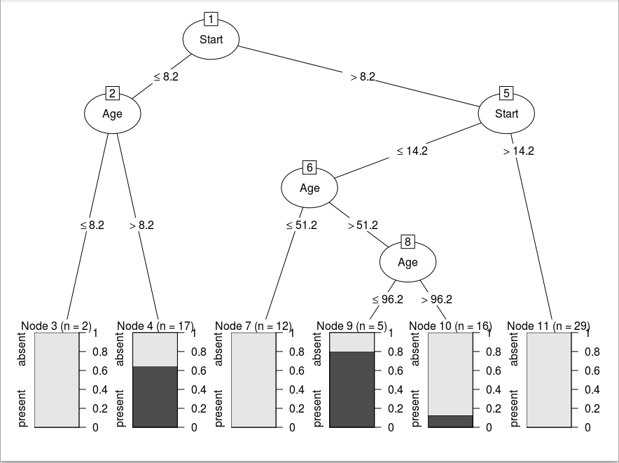
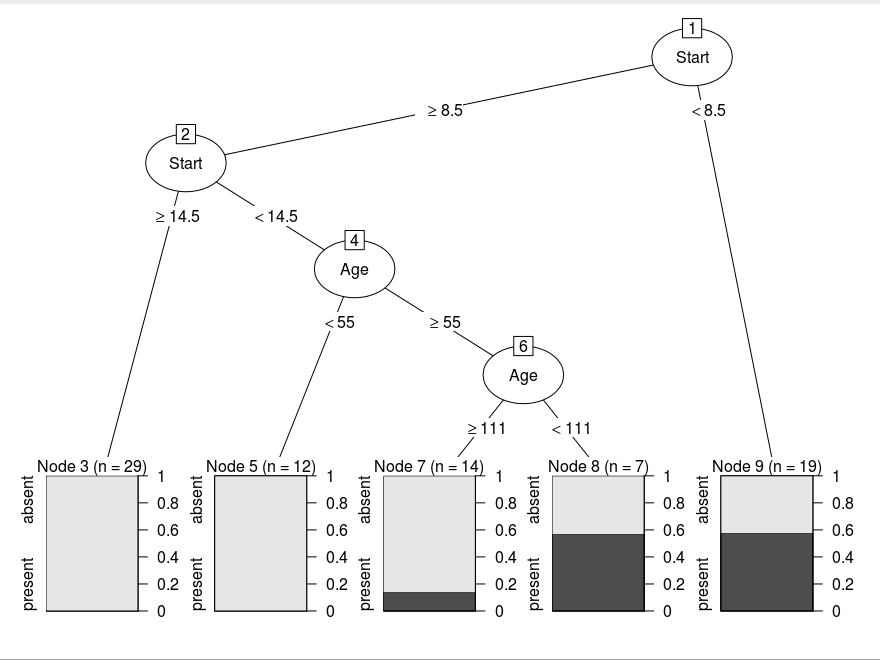
The rpart’s Desicion Tree
Iris
The dataset Iris
The b_index table and The new generated Tree.
##    id varid break terminal kidi kidf       info   tag
## 1   1     4     2        0   11    2             root
## 2   2     5   1.8        0   10    3 versicolor right
## 3   3     4     5        0    5    4  virginica right
## 4   4     0     0        1    0    0  virginica right
## 5   5     0     0        1    0    0  virginica  left
## 6   6     4     5        0    6    7 versicolor  left
## 7   7     5   1.6        0    9    8  virginica right
## 8   8     0     0        1    0    0 versicolor right
## 9   9     0     0        1    0    0  virginica  left
## 10 10     0     0        1    0    0 versicolor  left
## 11 11     0     0        1    0    0     setosa  left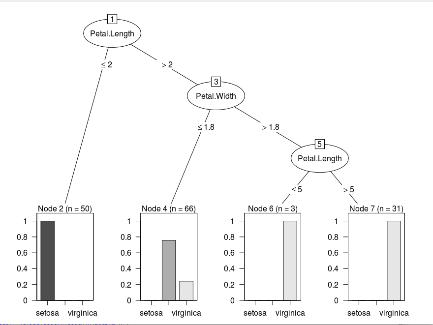
The rpart’s Desicion Tree
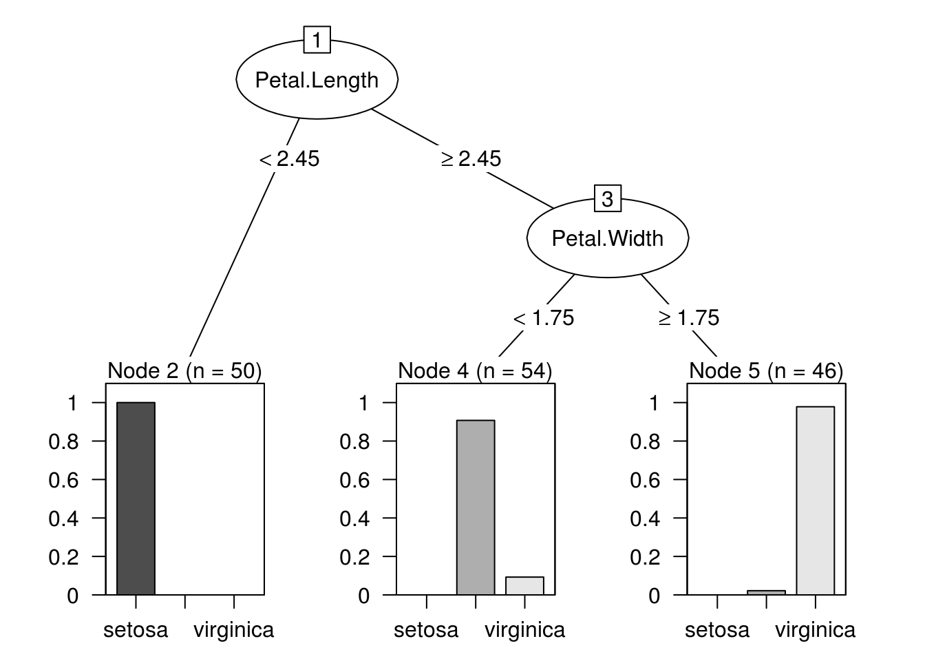
We can see that the splitting points are almost at same feature and point. The difference which is occuring is because rpart uses rescaled gini methods (which behaves like hybrid of gini and information gain methods) for cost function and we are using only gini index as cost function.